Linear Regression

A Line That Predicts

Imagine you track your electricity bill against the daily high temperature outside.

Hotter days mean your air conditioner runs longer, and the bill climbs. Plot those pairs and a trend appears.

Linear regression is the process of drawing the most accurate straight line through those data points.

Once the line exists, a new temperature reading gives you an instant cost estimate.

Input, Output, Relationship

Every regression starts with two roles.

The input is what you already know, such as the time spent cooking. The output is what you want to predict, such as the temperature of the meal.

Linear regression finds the most accurate relationship between that input and that output using one simple equation.

Nothing else is needed to begin.

The Shape of the Line

A straight line needs only two numbers.

One number sets how steep the line is. The other sets where the line sits when the input is zero.

Together they form the line of best fit:

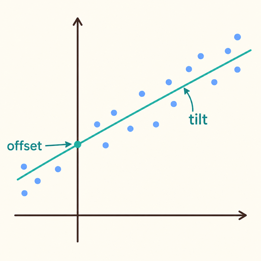
Notice that the tilt of the line is set by the weight while the height where it meets the vertical axis is set by the offset.

$$y = wx + b$$

In linear algebra terms, you are solving for a set of weights that describe the whole relationship.

Measuring How Wrong You Are

A guessed line is not enough. You need to score it.

For every data point, compare the value your line predicts against the value you actually observed. The gap between them is the error.

A cost function collects all those gaps into one number that measures how wrong the whole line is.

A small number means a good fit.

Adjust Until Error Shrinks

Fitting a line is not one calculation. It repeats.

You start with a line, measure the error, adjust the weights, and measure again.

Each pass should make the error smaller than the pass before it.

You stop when the error is as small as it can get. That final line is the line of best fit.

Guessing Versus Fitting

It is tempting to eyeball a line through your points and call it done.

That guess has no score behind it. You cannot tell whether a different line would be better.

Fitting replaces judgement with measurement. The cost function decides which line wins.

This is the difference between a hunch and a tool you can trust with a new reading.

Using the Fitted Line

Once the weights settle, prediction becomes cheap.

Take a new temperature reading, put it into the equation, and read out the estimated energy cost.

No searching through old bills is required. The line already carries what those bills taught it.

That is how raw historical data becomes a working tool.

What the Line Cannot Promise

The fitted line gives an estimate, not a guarantee.

Even the best line still has some error left over, because real points rarely sit perfectly on any straight path.

The cost function tells you how small that leftover error is.

A prediction is useful when you also know how far off it typically lands.

Putting It Together

Linear regression turns matrix equations into a prediction tool you can actually use.

You collect paired observations, draw a line, score it with a cost function, and adjust the weights until the error is as small as possible.

The result estimates energy cost from temperature, or meal temperature from cooking time.

Historical data becomes a plan for budgeting and managing resources.

In a linear regression model that predicts meal temperature from cooking time, is cooking time the input?

• Yes
• No

Answer: Yes

Yes. The input is the value already known or measured. Here, cooking time is known, while meal temperature is the output to predict.

In a line written as $$y = wx + b$$, $$w$$ determines the _____, while $$b$$ determines the _____ when $$x$$ is zero.

Answer: In a line written as $$y = wx + b$$, $$w$$ determines the steepness, while $$b$$ determines the position when $$x$$ is zero.

The weight $$w$$ controls how sharply the line rises or falls. The value $$b$$ sets the line's location at zero input.

Which description best matches the line of best fit in linear regression?

• The straight line with the smallest overall prediction error
• A straight line that passes through every observed point
• A line chosen only by visually estimating the trend
• A horizontal line that ignores the input values

Answer: The straight line with the smallest overall prediction error

The line of best fit is the straight line that represents the data most accurately, based on the size of its prediction errors. It does not need to pass through every point.